Introduction to neural networks
After we took a look at the different algorithms in the introduction to machine learning chapter we want to take a look at some special kind of machine learning algorithms which are called neural networks. This documents sikps the math part of neural networks in order to demonstrate those quickly. Those artifical neural networks were invented in the middle of the 20th century but due to the massive amount of data and computation needed for them to work they were put on the shelf until the beginnig of 21st century when such companies as Google collected much data and the GPU development increased rapidly thanks to the gaming industry.
The hello world of more advanced machine learning problems is the MNIST dataset, where e.g. a more basic but still interesting dataset is the Californa Housing dataset. The California Housing dataset can somehow tackled with linear regression, but problems like MNIST need much more context of each variable, which we call a dependent variable in statistics. One could say that the more dependent a variable is, the harder the problem.
As neural networks tend to be complex and demanding on the computational side there emerged some libraries in Python which allow to setup and train such networks, where the 2 biggest frameworks are TensorFlow by Google and PyTorch by Facebook. For this seminar we will focus on TensorFlow. These libraries are somehow quite similiar to SuperCollider as they allow to describe a graph of matehmatical operations via a high-level language (Python/sclang) which is then executed in the more performant language C++. Although they are somehow similar they have a different purpose: SuperCollider tries to calculate an audio stream in real time (which means we need to be fast as we do not have much time for the calculation) where TensorFlow needs to transport Gigabytes of data within secounds to multiple special devices like GPU or TPU. Also there are some algorithms implemented in TensorFlow which are missing in scsynth, such as the much important autodiff algorithm which makes neural networks feasible.
Although TensorFlow is a alread a Python library for the complicated C++ library there is a libary on top of TensorFlow which is called Keras which became the default library to interact with TensorFlow as writing native TensorFlow code can be exhausting.
Keep in mind that we are using TensorFlow 2 which is not compatible with TensorFlow (1) if you look up some examples online.
Like always we start with our imports, but now extended with tensorflow and keras (which comes bundled with tensorflow). If the import fails make sure to check the update procedure of the course material as tensorflow was originally not a dependency for this course and therefore needs to be installed manually in such a case. Check the docs on how to do this.
import numpy as np
import pandas as pd
import matplotlib.pyplot as plt
import tensorflow as tf
from tensorflow.keras import backend as K

np.random.seed(42) # make the results reproducible
Loading the MNIST dataset
Now its time to once again load the MNIST dataset which is mostly used to train a classifier to identify handwritten digits.
We can use keras for this.
Note that we already get a dataset which is split in x (the input, in our case the \(28 \times 28\) images) and y (the target, in our case the digit we want to predict) as well as train and test set (for serious working we would need a validation dataset as well).
We must hide the test set from the neural network during its training phase so we can evaluate how well the neural networks performs on example it has not seen before.
This is extremly important as the goal is to train a network which generalizes and not just work on input it already knows (which would be useless) which may sound trivial as a human but is suprisingly difficult to achieve this.
(x_train, y_train), (x_test, y_test) = tf.keras.datasets.mnist.load_data()
As always it is good to get familiar with the data in order to know what kind of structure the data is in and if it matches our expectations or if we made some error during loading and parsing of the data. On a real life example one would perform extensive statistical analysis on the dataset in order to ensure it lies within the expected order of deviations.
for name, array in zip(["x_train", "y_train", "x_test", "y_test"], [x_train, y_train, x_test, y_test]):
	print(f"Shape of {name}:\t{array.shape}")
Shape of x_train:	(60000, 28, 28)
Shape of y_train:	(60000,)
Shape of x_test:	(10000, 28, 28)
Shape of y_test:	(10000,)
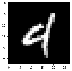
random_index = np.random.randint(x_train.shape[0])

plt.imshow(x_train[random_index], cmap='gray')
print(f"Label of example #{random_index} is {y_train[random_index]}")
Label of example #56422 is 4
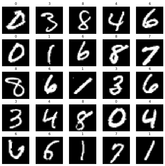
n_rows=5
n_cols=5
fig, axs = plt.subplots(n_rows, n_cols, figsize=(10, 10))
for i, idx in enumerate(np.random.randint(0, x_train.shape[0], n_rows*n_cols)):
    ax = axs[i%n_rows][i//n_rows]
    ax.imshow(x_train[idx], cmap='gray')
    ax.set_title(y_train[idx])
    ax.axis('off')
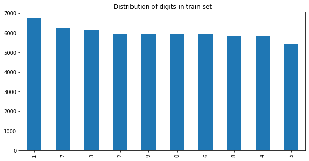
pd.Series(y_train).value_counts().plot.bar(title="Distribution of digits in train set", figsize=(10, 5));
Creating our first neural network
After we quickly analyzed the files we want to use for traning it is now time to write our first neural network. We will decide for a fully connected neural network (also called densely connected NN) as this is the most basic neural network. In a FCNN we create layers of neurons where each neuron of the layer is connected with each neuron of the following layer.
The graphic shows for example a neural network with one (also called hidden layer).

Source: https://commons.wikimedia.org/wiki/File:Colored_neural_network.svg
We start on the left side with a flat input vector and where each of the vectors scalar is connected with each scalar/neuron of the next layer. This connection often includes an activation function which allows the (de-)activation of neurons. This hidden layer is then connected with the output layer but could also be connected with another layer which allows to represent more complicated neuronal connections.
In the case of MNIST dataset our input is an image with \(28 \times 28\) pixels which each have a value between \(0\) (black) and \(255\) (white). As a vector needs to be 1-dimensional we simply flatten this image, so we obtain a \(28*28=784\) dimensional vector. The output of our neural network system is not the predicted number directly but the probability for each digit according to the neural network which results in a 10 dimensional output vector as we have 10 digits (from 0 to 9). Wo do this because the neural network can learn much better this way as we can describe mathematically more easily what we are searching for.
Our neural network is therefore much like a probibilty density function which shall output the proper digit according to its input.
During training we will tell the neural network that the best solution for an handwritten 2 as input should be the vector [0, 0, 1, 0, 0, 0, 0, 0, 0, 0].
This notation is also called one-hot-encoding which is often used for categorical problems.
Engouh talk, lets use kears to write a NN with one layer with 40 neurons.
model = tf.keras.models.Sequential([
    tf.keras.layers.Flatten(input_shape=(28, 28)), # our 28x28 image gets flattened
    tf.keras.layers.Dense(40), # the (hidden) layer
    tf.keras.layers.Dense(10), # the 10 dimensional output vector
])
Seems not so hard and keras also allows us to simply inspect the model as well.
model.summary()
Model: "sequential"
_________________________________________________________________
 Layer (type)                Output Shape              Param #
=================================================================
 flatten (Flatten)           (None, 784)               0

 dense (Dense)               (None, 40)                31400

 dense_1 (Dense)             (None, 10)                410

=================================================================
Total params: 31,810
Trainable params: 31,810
Non-trainable params: 0
_________________________________________________________________
Just a quick remark on the number of parameters. Our input layer has no trainable parameters as we shall not modify the input.
As every neuron of the input layer is connected with every neuron of our hidden layers the number of parameters grow rapidly:
The missing \(40\) parameters are due to the bias neuron which get added for each layer for mathematical reasions.
The next layer has
parameters - in this case we already included the additional bias neuron.
Training a neural network
For now we only iniated some matrices and vectors and connected them in a somehow senseful manner, yet we have now discussed how the computer really learns the neural network.
For this we will need to define a goal when a neural networks performs good or not via a so called loss-function (also called cost-function) which will tell us how good the neural network is performing right now. We can then calculate a gradient for the cost function with the parameter space of our neural networks as input which will tell us in which direction to modify the parameters of our neural network in order to get better results (this step is is actually not trivial but tensorflow helps us here).
In our case we use some knowledge from information theory to construct a good loss function and use an off-the-shelve optimizer from the keras library which drives the calculation of the derivative and applies the change in the parameterspace.
model.compile(
    optimizer=tf.keras.optimizers.Adam(),
    loss=tf.keras.losses.SparseCategoricalCrossentropy(from_logits=True),
    metrics='accuracy',
)
After all is said and done we can finally train our first neural network.
model.fit(x=x_train, y=y_train, epochs=5)
Epoch 1/5
1875/1875 [==============================] - 2s 796us/step - loss: 10.5197 - accuracy: 0.8514
Epoch 2/5
1875/1875 [==============================] - 1s 796us/step - loss: 3.4047 - accuracy: 0.8784
Epoch 3/5
1875/1875 [==============================] - 1s 791us/step - loss: 1.0116 - accuracy: 0.8836
Epoch 4/5
1875/1875 [==============================] - 2s 828us/step - loss: 0.5160 - accuracy: 0.8802
Epoch 5/5
1875/1875 [==============================] - 1s 785us/step - loss: 0.5351 - accuracy: 0.8725
<keras.callbacks.History at 0x162eee790>
We remember that we need to check the perfomance of our neural network on examples that it has not seen during training where the test set comes into play.
model.evaluate(x=x_test, y=y_test)
313/313 [==============================] - 0s 598us/step - loss: 0.6544 - accuracy: 0.8518
[0.6544067859649658, 0.8518000245094299]
We get an accuracy of about 87% which is already quite good but we can do better by applying some data pre-processing, making it easier for the algorithm to find good parameters in our neural network.
Tuning the neural network
Currently our input parameters (the brightness of each pixel) is between 0 and 255. Transforming this to be between 0 and 1 our algorithm can already learn faster as it is used to these kind of values.
x_train_scaled = x_train/255.0
x_test_scaled = x_test/255.0
We will also add a so called dropout layer and add another hidden layer and just apply all the same steps from above on our new model.
model_scaled = tf.keras.models.Sequential([
    tf.keras.layers.Flatten(input_shape=(28, 28)),
    tf.keras.layers.Dense(48, activation='relu'),
    tf.keras.layers.Dropout(0.3),
    tf.keras.layers.Dense(15),
    tf.keras.layers.Dropout(0.3),
    tf.keras.layers.Dense(10),
])

model_scaled.compile(
    optimizer=tf.keras.optimizers.Adam(),
    loss=tf.keras.losses.SparseCategoricalCrossentropy(from_logits=True),
    metrics='accuracy'
)
model_scaled.summary()
Model: "sequential_1"
_________________________________________________________________
 Layer (type)                Output Shape              Param #
=================================================================
 flatten_1 (Flatten)         (None, 784)               0

 dense_2 (Dense)             (None, 48)                37680

 dropout (Dropout)           (None, 48)                0

 dense_3 (Dense)             (None, 15)                735

 dropout_1 (Dropout)         (None, 15)                0

 dense_4 (Dense)             (None, 10)                160

=================================================================
Total params: 38,575
Trainable params: 38,575
Non-trainable params: 0
_________________________________________________________________
model_scaled.fit(x_train_scaled, y_train, epochs=5)
Epoch 1/5
1875/1875 [==============================] - 2s 899us/step - loss: 0.5824 - accuracy: 0.8214
Epoch 2/5
1875/1875 [==============================] - 2s 932us/step - loss: 0.3441 - accuracy: 0.9002
Epoch 3/5
1875/1875 [==============================] - 2s 866us/step - loss: 0.2957 - accuracy: 0.9127
Epoch 4/5
1875/1875 [==============================] - 2s 875us/step - loss: 0.2712 - accuracy: 0.9210
Epoch 5/5
1875/1875 [==============================] - 2s 874us/step - loss: 0.2526 - accuracy: 0.9272
<keras.callbacks.History at 0x163661700>
model_scaled.evaluate(x_test_scaled, y_test)
313/313 [==============================] - 0s 630us/step - loss: 0.1380 - accuracy: 0.9597
[0.13801522552967072, 0.9596999883651733]
Although we only added a few parameters and modified the training behaviour our model already performs better already. Now its time to take a look on the examples where our neural networks fail in order to get some new insights of the mechanics.
Analysing the results
We start by taking a look how we can ask the neural network for a prediction.
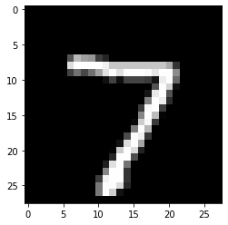
random_test_image_index = 0

plt.imshow(x_test_scaled[random_test_image_index], cmap='gray')
print(f"Label for image is {y_test[random_test_image_index]}")
Label for image is 7
We simply give the neural network the whole list of test images we have and ask for its probability of each class.
preds = model_scaled.predict(x_test_scaled)
preds[random_test_image_index]
array([ -2.8263762 ,   0.03036575,   6.4564805 ,   8.375091  ,
        -2.5378463 ,   4.2385798 , -11.81926   ,  20.765867  ,
        -3.2129931 ,   3.379484  ], dtype=float32)
pd.Series(preds[random_test_image_index]).plot.bar(
	title="Predicted probability for each digit class",
	grid=True,
);
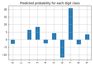
The neural network predicts our example correctly as a \(7\). We can use the argmax function in numpy to get the index with the highest value in a vector. And as we already have all predictions available we can perform this on every prediction also easily.
preds_one_hot = np.argmax(preds, axis=1)
This allows us to filter out the examples where the prediction did not work out as hoped.
false_indices = np.argwhere(preds_one_hot != y_test)
pd.Series(y_test[false_indices].flatten()).value_counts().plot.bar(
	title="Number of wrong predictions per class",
	grid=True,
);
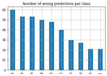
We see that our neural network seems to detect a \(0\) quite good (although it is also easy as it just needs to check if there are any pixels in the middle of the picture) but not great on a \(8\). But this analysis does not tell us for what the \(8\) got mistakenly taken for, but a confusion matrix can help us out here. Thankfully such things are build into TensorFlow.
From the docs we can obtain
The matrix columns represent the prediction labels and the rows represent the real labels.
If our neural network would work perfect we would obtain a diagonal matrix.
confusion_matrix = tf.math.confusion_matrix(y_test, preds_one_hot)
confusion_matrix
<tf.Tensor: shape=(10, 10), dtype=int32, numpy=
array([[ 959,    0,    0,    1,    0,    5,    9,    3,    3,    0],
       [   0, 1114,    2,    4,    0,    2,    3,    1,    9,    0],
       [   5,    3,  972,   16,    6,    1,    4,    9,   16,    0],
       [   0,    0,    1,  980,    0,   10,    0,   10,    6,    3],
       [   1,    0,    2,    0,  929,    0,   10,    1,    3,   36],
       [   5,    1,    0,   24,    0,  844,    5,    2,    4,    7],
       [   7,    3,    1,    1,    3,    8,  931,    0,    4,    0],
       [   1,    6,   17,    4,    1,    0,    0,  988,    1,   10],
       [   4,    1,    3,    8,    6,    7,    8,    8,  924,    5],
       [   3,    6,    0,   13,   13,    9,    1,    6,    2,  956]],
      dtype=int32)>
Lets take a closer look at some examples where the neural network predicted wrong.
n_rows=7
n_cols=7
fig, axs = plt.subplots(n_rows, n_cols, figsize=(15, 15))
for i, idx in enumerate(np.random.choice(false_indices.flatten(), n_rows*n_cols)):
    ax = axs[i%n_rows][i//n_rows]
    ax.imshow(x_test[idx], cmap='gray')
    ax.set_title(f'{preds_one_hot[idx]} (true: {y_test[idx]})')
    ax.axis('off')
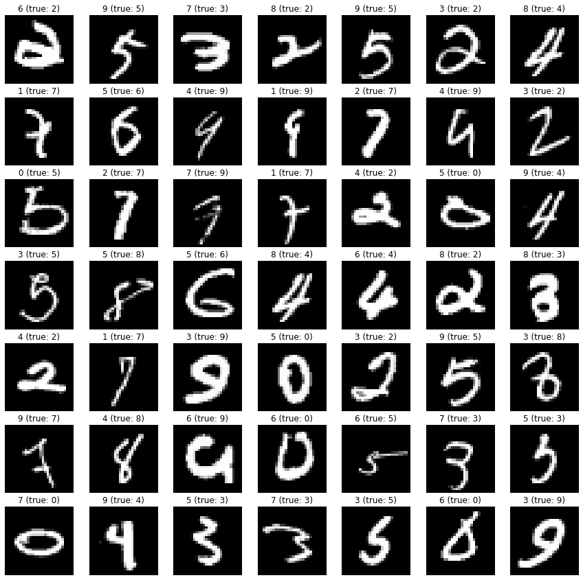
We see that some digits are indeed not clearly written and may be guessed wrongly by the human as well. Also it turns out that those classic datasets itself contain errors in its labeling as well, see labelerrors.com and [NAM21].
Therefore having a success rate of \(100\%\) on a machine learning problem is always sketchy and most likely occurs due to leakage of the y-labeled data into the input variable X.