Machine Learning basics¶

Now its time to take a look at the first machine learning algorithms. Thanks to the third-party library scikit-learn, also called sklearn, we can quickly use and exchange machine learning algorithms to solve tasks - even without understanding the inner mechanics of these algorithms, although it is advantageous to understand the inner mechanics of each algorithm to choose the best algorithm for each problem.

A recommended general read read is [Ger19] which will cover more details on using machine learning algorithms with sklearn.

import numpy as np
import pandas as pd
import matplotlib.pyplot as plt
from sklearn.datasets import fetch_openml

# mute sklearn warnings for cleaner output
def warn(*args, **kwargs):
    pass
import warnings
warnings.warn = warn

np.random.seed(42)

%matplotlib inline

Datasets¶

Machine learning is a discipline in which we do not give the computer a manual (also called an algorithm) to directly calculate the solution of a problem but instead give the computer data to look at in order to come up with good parameters for an algorithm which solves the problem. The algorithms we can use for this task can be a simple linear regression or can be a deep neural network. The decission which one to use is mostly determind by the complexity of our problem, but this can be a trap as demonstrated by the no free lunch theorem.

In order to calculate the best parameters for an algorithm we use data from a dataset and we also need a measure the performance of the algorithm which will be the target of our algorithm we want to optimize. One of the most famous datasets, the hello world of machine learning, is the MNIST dataset, which is a collection pictures of 70’000 images of handwritten digits with the labels which number is represented by the image.

We can use openml with scikit-learn to download and access the dataset.

mnist = fetch_openml('mnist_784', version=1)
print(mnist.DESCR)

**Author**: Yann LeCun, Corinna Cortes, Christopher J.C. Burges  
**Source**: [MNIST Website](http://yann.lecun.com/exdb/mnist/) - Date unknown  
**Please cite**:  

The MNIST database of handwritten digits with 784 features, raw data available at: http://yann.lecun.com/exdb/mnist/. It can be split in a training set of the first 60,000 examples, and a test set of 10,000 examples  

It is a subset of a larger set available from NIST. The digits have been size-normalized and centered in a fixed-size image. It is a good database for people who want to try learning techniques and pattern recognition methods on real-world data while spending minimal efforts on preprocessing and formatting. The original black and white (bilevel) images from NIST were size normalized to fit in a 20x20 pixel box while preserving their aspect ratio. The resulting images contain grey levels as a result of the anti-aliasing technique used by the normalization algorithm. the images were centered in a 28x28 image by computing the center of mass of the pixels, and translating the image so as to position this point at the center of the 28x28 field.  

With some classification methods (particularly template-based methods, such as SVM and K-nearest neighbors), the error rate improves when the digits are centered by bounding box rather than center of mass. If you do this kind of pre-processing, you should report it in your publications. The MNIST database was constructed from NIST's NIST originally designated SD-3 as their training set and SD-1 as their test set. However, SD-3 is much cleaner and easier to recognize than SD-1. The reason for this can be found on the fact that SD-3 was collected among Census Bureau employees, while SD-1 was collected among high-school students. Drawing sensible conclusions from learning experiments requires that the result be independent of the choice of training set and test among the complete set of samples. Therefore it was necessary to build a new database by mixing NIST's datasets.  

The MNIST training set is composed of 30,000 patterns from SD-3 and 30,000 patterns from SD-1. Our test set was composed of 5,000 patterns from SD-3 and 5,000 patterns from SD-1. The 60,000 pattern training set contained examples from approximately 250 writers. We made sure that the sets of writers of the training set and test set were disjoint. SD-1 contains 58,527 digit images written by 500 different writers. In contrast to SD-3, where blocks of data from each writer appeared in sequence, the data in SD-1 is scrambled. Writer identities for SD-1 is available and we used this information to unscramble the writers. We then split SD-1 in two: characters written by the first 250 writers went into our new training set. The remaining 250 writers were placed in our test set. Thus we had two sets with nearly 30,000 examples each. The new training set was completed with enough examples from SD-3, starting at pattern # 0, to make a full set of 60,000 training patterns. Similarly, the new test set was completed with SD-3 examples starting at pattern # 35,000 to make a full set with 60,000 test patterns. Only a subset of 10,000 test images (5,000 from SD-1 and 5,000 from SD-3) is available on this site. The full 60,000 sample training set is available.

Downloaded from openml.org.

We can access the image data via the .data attribute of the dataset which yields a pandas dataframe which is similar to an Excel spreadsheet.

mnist.data

	pixel1	pixel2	pixel3	pixel4	pixel5	pixel6	pixel7	pixel8	pixel9	pixel10	...	pixel775	pixel776	pixel777	pixel778	pixel779	pixel780	pixel781	pixel782	pixel783	pixel784
0	0.0	0.0	0.0	0.0	0.0	0.0	0.0	0.0	0.0	0.0	...	0.0	0.0	0.0	0.0	0.0	0.0	0.0	0.0	0.0	0.0
1	0.0	0.0	0.0	0.0	0.0	0.0	0.0	0.0	0.0	0.0	...	0.0	0.0	0.0	0.0	0.0	0.0	0.0	0.0	0.0	0.0
2	0.0	0.0	0.0	0.0	0.0	0.0	0.0	0.0	0.0	0.0	...	0.0	0.0	0.0	0.0	0.0	0.0	0.0	0.0	0.0	0.0
3	0.0	0.0	0.0	0.0	0.0	0.0	0.0	0.0	0.0	0.0	...	0.0	0.0	0.0	0.0	0.0	0.0	0.0	0.0	0.0	0.0
4	0.0	0.0	0.0	0.0	0.0	0.0	0.0	0.0	0.0	0.0	...	0.0	0.0	0.0	0.0	0.0	0.0	0.0	0.0	0.0	0.0
...	...	...	...	...	...	...	...	...	...	...	...	...	...	...	...	...	...	...	...	...	...
69995	0.0	0.0	0.0	0.0	0.0	0.0	0.0	0.0	0.0	0.0	...	0.0	0.0	0.0	0.0	0.0	0.0	0.0	0.0	0.0	0.0
69996	0.0	0.0	0.0	0.0	0.0	0.0	0.0	0.0	0.0	0.0	...	0.0	0.0	0.0	0.0	0.0	0.0	0.0	0.0	0.0	0.0
69997	0.0	0.0	0.0	0.0	0.0	0.0	0.0	0.0	0.0	0.0	...	0.0	0.0	0.0	0.0	0.0	0.0	0.0	0.0	0.0	0.0
69998	0.0	0.0	0.0	0.0	0.0	0.0	0.0	0.0	0.0	0.0	...	0.0	0.0	0.0	0.0	0.0	0.0	0.0	0.0	0.0	0.0
69999	0.0	0.0	0.0	0.0	0.0	0.0	0.0	0.0	0.0	0.0	...	0.0	0.0	0.0	0.0	0.0	0.0	0.0	0.0	0.0	0.0

70000 rows × 784 columns

Before we take a look at how to interpret and display the handdrawn images we will take a look at the labels associated with each image which are stored in the .target attribute.

mnist.target

      5
      0
      4
      1
      9
        ..
  2
  3
  4
  5
  6
Name: class, Length: 70000, dtype: category
Categories (10, object): ['0', '1', '2', '3', ..., '6', '7', '8', '9']

We observe that the labels are not integers but categories (see dtype: category) - we will fix this immediately by transforming the categories to integers using astype. This is a pandas specific way to save memory but we can live with storing 70’000 integers in an array.

mnist.target = mnist.target.astype(np.int8)
mnist.target

      5
      0
      4
      1
      9
        ..
  2
  3
  4
  5
  6
Name: class, Length: 70000, dtype: int8

We will also create another label which determines if the shown handrawn digit is a 5 or not as the prediction if some digit is a 5 or not is a simpler problem than to determine which digit is shown. Normally we would use a binary label for this but as we are working in a numerical domain we will use the encoding False = 0 and True = 1. For the conversion we can use astype(int).

y_just_5 = (mnist.target==5).astype(np.int8)
y_just_5

      1
      0
      0
      0
      0
        ..
  0
  0
  0
  1
  0
Name: class, Length: 70000, dtype: int8

Visualising the data¶

Its always a good practice to visualise the dataset in order to get an understanding of it. Lurking through everyone of the 70000 samples is a tedious work, although it maybe worth it. Instead we will use methods of statistical analysis to shrink down our data to something more easily observable.

We can convert the .data stored in a pandas dataframe to a numpy array which makes it easier for us to work with the data.

mnist_data = mnist.data.to_numpy()
mnist_data.shape

(70000, 784)

As the images have a square format we can use \(\sqrt{784} = 28\) to determine that we need to reshape our single line of pixels to a \(28\times28\) matrix. We can use the reshape function of numpy to transfer our 784 dimensional vector to such a matrix, where -1 is used as a free radical which will be determind automatically based on the given structure.

mnist_reshaped = mnist_data.reshape(-1, 28, 28)
mnist_reshaped.shape

(70000, 28, 28)

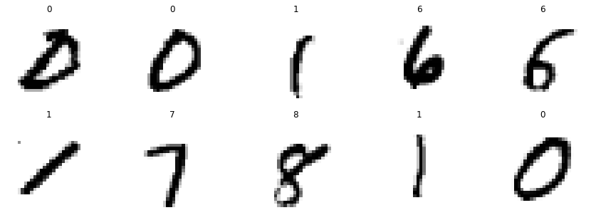
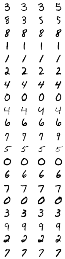
We can now easily plot 10 random images with its according label.

plt.figure(figsize=(15, 5));
for i, index in enumerate(np.random.choice(mnist_reshaped.shape[0], 10)):
    plt.subplot(2, 5, i+1)
    plt.axis('off')
    plt.imshow(mnist_reshaped[index, :, :], cmap='binary')
    plt.title(f'{mnist.target[index]}')
plt.show()

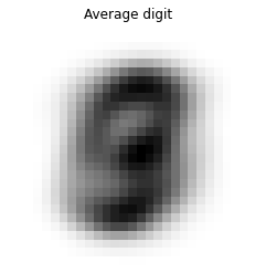
Mean¶

We can also take a look at the average handdrawn digit from the MNIST dataset by meaning the pixels over all examples we have. Because we only want to calculate the average image from all available images we do not want to take the mean of all pixels (which would result in a single pixel) but only the mean along one dimension (the dimension of \(n\)-examples) which is our first dimension of our \(70'000 \times 28 \times 28\) matrix so that we have a meaned matrix of dimension \(28 \times 28\).

plt.title('Average digit')
plt.axis('off')
plt.imshow(np.mean(mnist_reshaped, axis=0), cmap='binary');

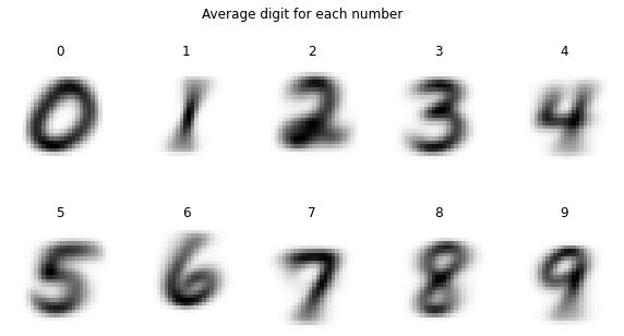
We can make this more interesting by not meaning over all digits but only calculating a mean for each class of numbers in our dataset.

plt.figure(figsize=(10, 5))
for i in range(0, 10):
    plt.subplot(2, 5, i+1)
    plt.axis('off')
    plt.imshow(np.mean(mnist_reshaped[(mnist.target==i), :, :], axis=0), cmap='binary')
    plt.title(f'{i}')
plt.suptitle('Average digit for each number')
plt.show()

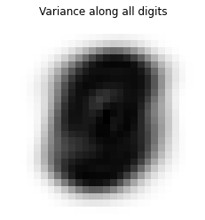
Variance¶

Mean is not the only metric that statistics gives us to inspect data. Variance is another practical metric and tells us for each pixel if the value is fluctuiating throughout the examples a lot (high variance) or if its not changing at all throughout the examples (variance = 0). If the variance of a pixel is 0 it gives us not any information about the number it represents because the value of the pixel is the same for all examples so there is no way to distinguish the numbers by looking at this pixel.

plt.imshow(np.var(mnist_reshaped, axis=0), cmap='binary')
plt.axis('off')
plt.title('Variance along all digits')
plt.show();

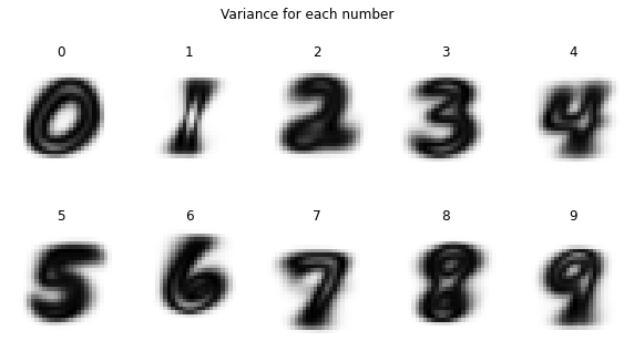
We can also take a look at the variance within each class of numbers. This tells us which pixels differ over all examples within the same class (high variance, black) and which pixels are the same throughout the examples (low variance, white).

plt.figure(figsize=(10, 5))
for i in range(0, 10):
    plt.subplot(2, 5, i+1)
    plt.axis('off')
    plt.imshow(np.var(mnist_reshaped[(mnist.target==i), :, :], axis=0), cmap='binary')
    plt.title(f'{i}')
plt.suptitle('Variance for each number')
plt.show()

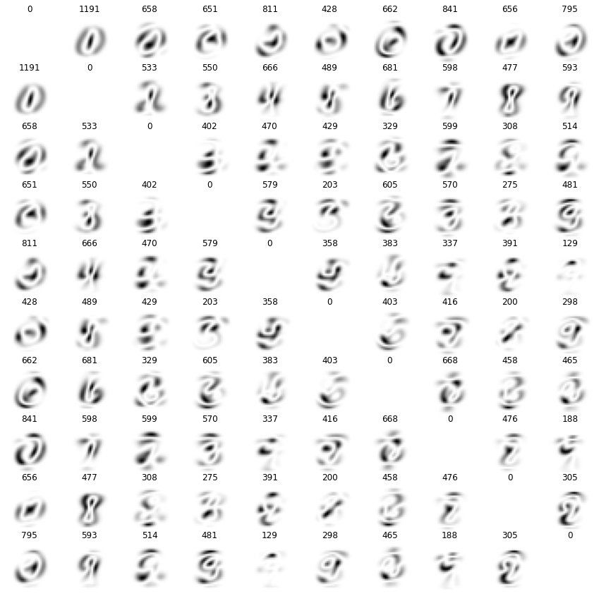
We can also compare the variance between two classes of numbers. This tells us which pixels are important to distinguish two classes of numbers. Above each variance plot is the meaned variance for the shown combination of classes - a high meaned variance means that the pixel values differ a lot when comparing the two classes and vice versa.

The \(i\)-th row represents the \(i\)-th number (starting at 0) and the \(j\)-th row the \(j\)-th number.

plt.figure(figsize=(15, 15))
fig, axs = plt.subplots(10, 10, figsize=(15, 15))
for i in range(0, 10):
    for j in range(0, 10):
        mean_i = np.mean(mnist_reshaped[(mnist.target==i)], axis=0)
        mean_j = np.mean(mnist_reshaped[(mnist.target==j)], axis=0)
        axs[i, j].imshow(np.var([mean_i, mean_j], axis=0), cmap='binary')
        axs[i, j].set_title(f'{np.mean(np.var([mean_i, mean_j], axis=0)):.0f}')
        axs[i, j].set_axis_off()
plt.show();

<Figure size 1080x1080 with 0 Axes>

Labels¶

Of course we also need to take a look at the labels - if some number is not represented equally it would make our problem harder because the algorithm could take the shortcut to always forecast the more likely number within our dataset.

mnist.target.value_counts().plot.bar(figsize=(10, 5), grid=True);
plt.title('# of examples for a class in the dataset');

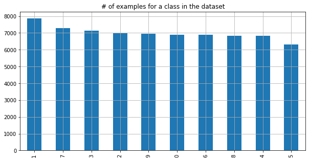
We see that the number of classes is quiet equally distributed, although we have over 1000 more examples of a 1 than of a 5. This gets more skewed if we take a look at our simpler problem by reducing the problem to detect if the shown image is a 5 or not.

y_just_5.value_counts().plot.bar(grid=True, figsize=(10, 5))
plt.title('# of examples which show 5');

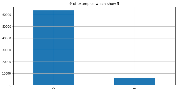
y_just_5.value_counts(normalize=True)

0    0.909814
1    0.090186
Name: class, dtype: float64

The data tells us that 90% of the data has the label “no 5” - if we define an algorithm which always returns False it is 90% right of the time but has not learned anything useful. We call this simple algorithm a baseline and often it is good practice to think of a good baseline before turning towards machine learning as thinking about the baseline reveals a lot of the problem which will be useful for solving the problem via machine learning as well and may make the use of machine learning obsolete.

Train/test split¶

In order to evaluate the performance of an algorithm we have to hide certain examples during the training stage of the algorithm (called training set) and then evaluate the performance of the algorithm on these hidden examples (called test set). Otherwise the algorithm could just remember all the examples from training and not learn how to solve the problem in general - but this generalisation is our goal.

sklearn provides a convenience function for the splitting of our datasets called train_test_split.

from sklearn.model_selection import train_test_split

X_train, X_test, y_train, y_test, y5_train, y5_test = train_test_split(mnist.data, mnist.target, y_just_5, train_size=0.7, shuffle=True, random_state=42)
print(f'X shape \t train: {X_train.shape} \t test: {X_test.shape}')
print(f'y shape \t train: {y_train.shape} \t test: {y_test.shape}')
print(f'y5 shape \t train: {y5_train.shape} \t test: {y5_test.shape}')

X shape 	 train: (49000, 784) 	 test: (21000, 784)
y shape 	 train: (49000,) 	 test: (21000,)
y5 shape 	 train: (49000,) 	 test: (21000,)

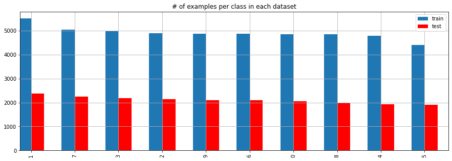
We should check if our traning and test set are somehow similliar in order to avoid that certain cases are missing in the traning set.

ax = y_train.value_counts().plot.bar(position=1, width=0.3, label='train', figsize=(15, 5))
y_test.value_counts().plot.bar(ax=ax, position=0, width=0.3, color='r', label='test', grid=True)
plt.legend()
plt.title('# of examples per class in each dataset')
plt.show();

Classification¶

One application and subset of machine learning is the classification of data. This can be detecting the number of the handdrawn digit on the MNIST dataset or mapping an image of a face to a name of a person (although real world examples use slightly different aproaches, see FaceNet).

In the early 2010s deep learning helped to make big steps in the discipline of automatic classification of data (especially thanks to convolutional neural networks which yield remarking results in pattern recognition) which also was later transformed to generate new data, called generative learning.

Training a classifier¶

sklearn provides a multitude of classifiers which all share the same interface so they are quickly interchangeable and comparable. The following code demonstrates how we can quickly train such a classifier although for a real machine learning project we are omitting a lot of useful and necessary steps (e.g. pre-processing, combining multiple classifiers called ensemble learning).

We will train two classifiers - a simple linear classifier and a more soffiscicated random forest.

from sklearn.linear_model import RidgeClassifier
from sklearn.ensemble import RandomForestClassifier
from sklearn.metrics import classification_report

# setting the random state makes the randomness deterministic
# obtaining the same results throughout multiple runs of the notebook
ridge = RidgeClassifier(random_state=42)
rf = RandomForestClassifier(random_state=42)

Traning a classifier is as simple as calling the .fit method with the data (also called features) and its target (also called labels). Based on the complexity of the used algorithm and the amount of data the training can either run on a notebook within a few seconds or need a cluster of high end computers for multiple weeks.

The used algorithms should be trained within a few minutes.

We will also take a look at the performance of both algorithms on our test set.

ridge = RidgeClassifier()
ridge.fit(X_train, y_train)

print(classification_report(y_test, ridge.predict(X_test)))

              precision    recall  f1-score   support

           0       0.90      0.95      0.92      2058
           1       0.80      0.97      0.88      2364
           2       0.90      0.79      0.84      2133
           3       0.82      0.84      0.83      2176
           4       0.81      0.89      0.85      1936
           5       0.87      0.72      0.79      1915
           6       0.90      0.92      0.91      2088
           7       0.88      0.86      0.87      2248
           8       0.83      0.74      0.78      1992
           9       0.82      0.80      0.81      2090

    accuracy                           0.85     21000
   macro avg       0.85      0.85      0.85     21000
weighted avg       0.85      0.85      0.85     21000

rf = RandomForestClassifier()
rf.fit(X_train, y_train)

print(classification_report(y_test, rf.predict(X_test)))

              precision    recall  f1-score   support

           0       0.98      0.98      0.98      2058
           1       0.98      0.98      0.98      2364
           2       0.96      0.97      0.96      2133
           3       0.96      0.95      0.95      2176
           4       0.96      0.97      0.97      1936
           5       0.97      0.96      0.96      1915
           6       0.98      0.98      0.98      2088
           7       0.97      0.97      0.97      2248
           8       0.96      0.95      0.95      1992
           9       0.95      0.95      0.95      2090

    accuracy                           0.97     21000
   macro avg       0.97      0.97      0.97     21000
weighted avg       0.97      0.97      0.97     21000

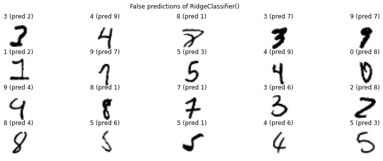
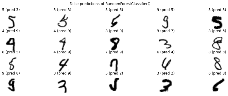
We see that our linear regression model has already an accuracy of \(85\%\), but the random forest easily surpasses this with an accuracy of \(97\%\) which is already really good. It is often worth to take a look at the examples that got predicted wrong.

for predictor in [ridge, rf]:
    pred = predictor.predict(X_test)
    false_pred_idx = np.where(pred!=y_test)[0]
    plt.figure(figsize=(15, 5))
    for i, false_idx in enumerate(np.random.choice(false_pred_idx, 20)):
        plt.subplot(4, 5, i+1)
        plt.imshow(X_test.to_numpy()[false_idx].reshape(28, 28), cmap='binary')
        plt.title(f'{y_test.iloc[false_idx]} (pred {pred[false_idx]})')
        plt.axis('off')
    plt.suptitle(f'False predictions of {predictor}')
    plt.show()

non-5 vs 5¶

Lets measure the performance of our simpler problem - although we here have the problem that we have way more examples of a non-5 than that of a 5, so only looking at the accuracy may will mislead us.

ridge_5 = RidgeClassifier(random_state=42)
ridge_5.fit(X_train, y5_train)

print(classification_report(y5_test, ridge_5.predict(X_test)))

              precision    recall  f1-score   support

           0       0.95      0.99      0.97     19085
           1       0.89      0.44      0.59      1915

    accuracy                           0.94     21000
   macro avg       0.92      0.72      0.78     21000
weighted avg       0.94      0.94      0.93     21000

rf_5 = RandomForestClassifier(random_state=42)
rf_5.fit(X_train, y5_train)

print(classification_report(y5_test, rf_5.predict(X_test)))

              precision    recall  f1-score   support

           0       0.99      1.00      0.99     19085
           1       0.99      0.88      0.93      1915

    accuracy                           0.99     21000
   macro avg       0.99      0.94      0.96     21000
weighted avg       0.99      0.99      0.99     21000

Remeber that our baseline could achive the following by just predicting that we never see a 5.

print(classification_report(y5_test, [0]*len(y5_test)))

              precision    recall  f1-score   support

           0       0.91      1.00      0.95     19085
           1       0.00      0.00      0.00      1915

    accuracy                           0.91     21000
   macro avg       0.45      0.50      0.48     21000
weighted avg       0.83      0.91      0.87     21000

With all classifiers we obtain an accuracy of over \(90\%\), but taking a look at the recall and precission of the detection of the 5 reveals us which algorithm actually performs good at the taks we want to solve. Where our baseline can not identify any of our examples of 5 and therefore fails at this task, the ridge regressor detected only \(44\%\) of the 5s properly and out of all the 5s it detected only \(89\%\) were actually a 5. Only \(1\%\) of all examples where the random forest claimed to detect a 5 were in reality not a 5 (\(99\%\) precision) and and detected \(87\%\) of all the 5s in the dataset.

The important bit to take away here is to understanding the metrics and the performance of a classification properly.

Regression¶

One big topic in machine learning is regression - instead of predicting the class of a certain example we want to calculate based in the input features another output vector. One example of regression would be the prediction of the water level of the Rhine based on weather data. We could also try to predict the water level by the number of released documentaries in cinemas for each week but there is the question of correlation vs causality.

We can use regression on our MNIST dataset to finish a partially shown digit. Based on the first 300 pixels we want to predict the remaining \((28*28)-300=484\) pixels. This means that we are using the first \(\frac{300}{784} \approx 38 \%\) of the image to predict the remaining \(\frac{484}{700} \approx 62 \%\).

from sklearn.linear_model import Ridge
from sklearn.multioutput import MultiOutputRegressor

sgdr = MultiOutputRegressor(Ridge())

sgdr.fit(X_train.to_numpy()[:, :300], X_train.to_numpy()[:, 300:])

MultiOutputRegressor(estimator=Ridge())

After we have fitted the regressor on our training data we can now try to continue examples from our traning set.

plt.figure(figsize=(15, 3))
for i, idx in enumerate(np.random.randint(len(X_test), size=10)):
    # plot original
    plt.subplot(2, 10, i+1)
    plt.imshow(X_test.to_numpy()[idx].reshape(28, 28), cmap='binary')
    plt.axis('off')
    # plot reconstructed
    plt.subplot(2, 10, 10+i+1)
    pred = sgdr.predict(X_test.to_numpy()[idx:idx+1, :300])
    canvas = np.zeros(shape=(28*28))
    canvas[:300] = X_test.to_numpy()[idx:idx+1, :300]
    canvas[300:] = pred[0]
    plt.imshow(canvas.reshape(28, 28), cmap='binary')
    plt.title('')
    plt.axis('off')
plt.show()

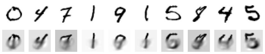
We can use a simple regressor to continue a given signal based on the signals we observed earlier - here it is the brightness of our pixels. Currently this is rather blurry because in our current aproach the prediction of each pixel is independent of one another, so the pixels next to each other do not interact with each other and share information about their result but this is maybe necessary as they depend on each other to properly represent a digit clearly. This is also amplified by the fact that we are representing the image as a single line of dots so their vertical realtionship gets lost (Convolutional Neural Networks try to tackle the last problem).

On the other hand we may are asking for an definitve answer for a problem which has ambigious answers as the first 300 pixels may contain too few information to come up with one precise continuation of the picture.

The detection of a partial and evolving drawing is also the inspiration for the project quickdraw.

Clustering¶

Another common application of machine learning is clustering. This is also an example of unsupervised learning as for the application of clustering we do not need any kind of labels as it would be otherwise an classification task. Having no need for labels is also the advantage of clustering algorithms which can be used for recommendation and categorisation of unlabeled data.

We can use sklearn here as it implements a variety of clustering algorithms. Lets say we do not know anything about our data but want to take a look at some examples the most distinct digits - we can cluster the MNIST pictures to \(n\) clusters using KMeans and take a look at the \(4\) closest representation of these instances by uisng NearestNeighbors.

from sklearn.cluster import KMeans

k_means = KMeans(n_clusters=20)
k_means.fit(mnist.data)

KMeans(n_clusters=20)

from sklearn.neighbors import NearestNeighbors

# use nearest neighbors to find the closest example to the center of our cluster
nn = NearestNeighbors(n_neighbors=4)
nn.fit(mnist.data)

plt.figure(figsize=(5, 20))
for i, cluster_center in enumerate(k_means.cluster_centers_):
    center_examples = nn.kneighbors(cluster_center[np.newaxis, :], return_distance=False)[0]
    for j, example in enumerate(center_examples):
        plt.subplot(20, 4, (4*i)+j+1)
        plt.imshow(mnist.data.to_numpy()[example].reshape(28, 28), cmap='binary')
        plt.axis('off')
plt.show()

Dimensionality reduction¶

As a last topic to cover in this quick introduction to machine learning is dimensionality reduction. When working with data we quickly exceed the human visible perceivable dimensions and are on top constrained by a 2 dimensional display of a computer most of the time while working on data analysis. To still gather a glimpse on this high dimensionality we can use dimensionality reduction algorithms to condense the information down to a more observable state. It is also often used as a pre-processing step on more complex algorithms to reduce the necessary amount of resources for calculation.

A common known dimensionality reduction is the occurence of shadows which map a 3 dimensional object onto a 2 dimensional plane. By moving the light source in the 3 dimensions we can modify the shadow - in this regard dimensionality reduction algorithms try to find a good position of our light source to preserve as much information as possible about the distance of each object to another object in the high dimension space. A common measurement for this is variance and is used by PCA, principal component analysis.

We can use these algorithms to display all 70’000 images of the MNIST dataset in a single plot by reducing the 784 dimensions of pixels down to 2 dimensions so each picture is represented by a single dot in a 2 dimensional space.

from sklearn.decomposition import PCA

pca = PCA(n_components=2)
mnist_2dim = pca.fit_transform(mnist_data)

fig = plt.figure(figsize=(15, 15))
scatter = plt.scatter(mnist_2dim[:, 0], mnist_2dim[:, 1], c=mnist.target.astype(int), cmap='nipy_spectral', s=2.0)
plt.legend(*scatter.legend_elements());

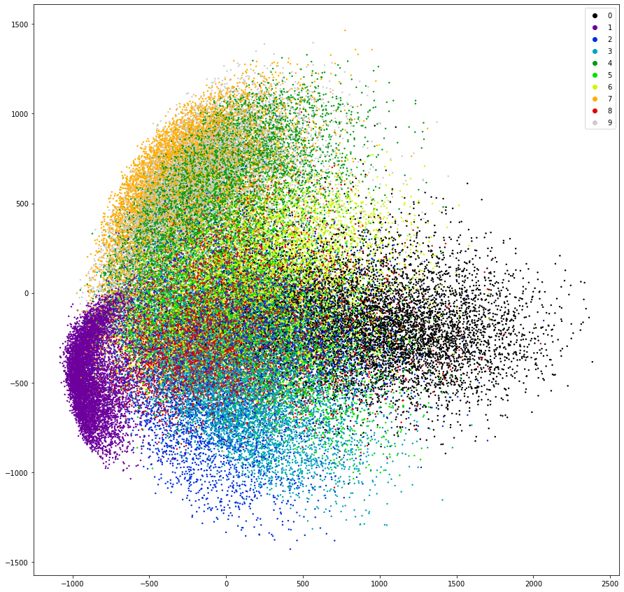
It is remarkable that PCA could already separate all digits of 1 (purple) into its own space just by looking at the variance of the data - PCA is also an unsupervised algorithm and as such does not need any labels. Also all images of the digit 7 got positioned close to the images of 1 (orange) which intuitively makes sense.

Another dimensionality reduction algorithm which works well for 2 or 3 dimensional representation of data is T-sne which is also implemented in sklearn but, due to its complexity, takes some minutes to calculate.

from sklearn.manifold import TSNE

tsne = TSNE(n_components=2, random_state=42)
mnist_2dim_tsne = tsne.fit_transform(mnist_data)

fig = plt.figure(figsize=(15, 15))
scatter = plt.scatter(mnist_2dim_tsne[:, 0], mnist_2dim_tsne[:, 1], c=mnist.target.astype(int), cmap='nipy_spectral', s=2.0)
plt.legend(*scatter.legend_elements());

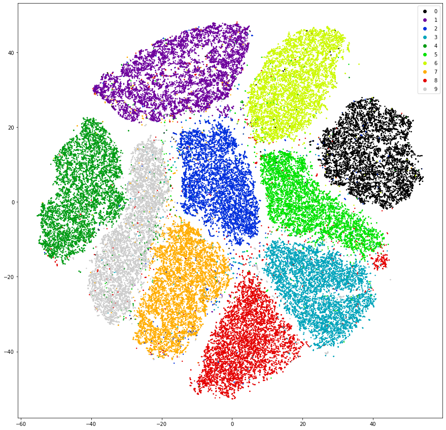
Using another algorithm on the same data yields much more promosing results. The clusters are much better separated and each cluster is less noisy compared to our PCA aproach. By drawing a line to segment each of the clusters we already would have made a good classification algorithm eventhough the dimensionality reduction algorithm never glimpsed at the underlying labels. Using these dimensionality reduction algorithms can also be used in an artistic way which we will explore in another notebook.

Musikinformatik SoSe2021